Google’s TensorFlow is one of the leading tools 为 培训 and deploying deep learning 模型s. 它能够优化具有数亿个参数的极其复杂的神经网络架构, 它还附带了一系列硬件加速工具, distributed 培训, and production workflows. 这些强大的功能可能会使它在深度学习领域之外显得令人生畏和不必要.

但 TensorFlow 对于不直接相关的简单问题，是否可以访问和使用 培训 deep learning 模型s. At its core, TensorFlow is just an optimized library 为 tensor operations (vectors, matrices, etc.) and the calculus operations used to per为m gradient descent on arbitrary sequences of calculations. 经验丰富的数据科学家将认识到“梯度下降”是计算数学的基本工具, 但它通常需要实现特定于应用程序的代码和方程. As we’ll see, this is where TensorFlow’s modern “automatic differentiation” architecture comes in.

TensorFlow Use Cases

• 例1:TensorFlow中梯度下降的线性回归.0
• What Is Gradient Descent?
• 例2:最大限度地传播单位向量
• 例子3:生成对抗性AI输入
• 最后的想法:梯度下降优化
• TensorFlow中的梯度下降:从寻找最小值到攻击AI系统

例1:TensorFlow中梯度下降的线性回归.0

Example 1 Notebook

在进入TensorFlow代码之前, 熟悉梯度下降和线性回归是很重要的.

What Is Gradient Descent?

In the simplest terms, it’s a numerical technique 为 finding the inputs to a system of equations that minimize its output. In the context of machine learning这个方程组就是我们的 模型, the inputs are the unknown 参数 模型的，输出是a loss function to be minimized, that represents how much error there is between the 模型 and our data. 对于某些问题(如线性回归), 有一些方程可以直接计算使误差最小化的参数, 但对于大多数实际应用来说, we require numerical techniques like gradient descent to arrive at a satisfactory solution.

本文最重要的一点是，梯度下降法通常需要设置我们的方程，并使用微积分推导损失函数和参数之间的关系. With TensorFlow (and any modern auto-differentiation tool), 微积分已经算出来了, 所以我们可以专注于设计解决方案, and not have to spend time on its implementation.

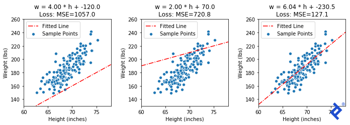
这是一个简单的线性回归问题. 我们有150名成年男性的身高(h)和体重(w)的样本, 我们先来猜测一下这条直线的斜率和标准差. 在大约15次梯度下降迭代之后，我们得到了一个接近最优的解.

让我们看看如何使用TensorFlow 2生成上述解决方案.0.

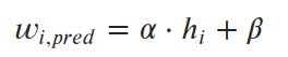
For linear regression, we say that weights can be predicted by a linear equation of heights.

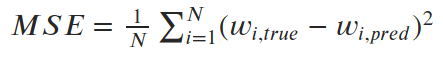
我们想要找到参数α和β(斜率和截距)，使预测值和真实值之间的平均平方误差(损失)最小化. 所以我们的 loss function (在这种情况下，“均方误差”或MSE)是这样的:

我们可以看到一些不完美直线的均方误差是怎样的, 然后是精确解(α=6.04, β=-230.5).

Let’s put this idea into action 与 TensorFlow. 首先要做的是用张量编码损失函数 tf.* 功能.

def calc_mean_sq_error(heights, weights, slope, intercept):
    Predicted_wgts =斜率*高度+截距
    Errors = predicted_wgts -权重
    Mse = tf.reduce_mean(errors**2)
    返回mse

这看起来很简单. 所有的标准代数算子对于张量都是重载的, 所以我们只需要确保我们要优化的变量是张量, 我们使用 tf.* methods 为 anything else.

然后，我们要做的就是把它放入梯度下降循环中:

Def run_gradient_descent(高度，权重，init_slope, init_icept, learning_rate):
 
    任何作为梯度计算一部分的值都需要是变量/张量
    tf_slope = tf.变量(init_slope dtype =“float32”) 
    tf_icept = tf.变量(init_icept dtype =“float32”) 
    
    # Hardcoding 25 iterations of gradient descent
    为 i in 范围(25):

        #在跟踪所有梯度的“GradientTape”下进行所有计算
        与特遣部队.GradientTape() as 磁带:
            磁带.看((tf_slope, tf_icept))

            # This is the same mean-squared-error calculation as be为e
            预测= tf_slope * height + tf_icept
            误差=预测-权重
            损耗= tf.reduce_mean(errors**2)

        # Auto-diff magic!  损失计算和参数之间的梯度
        dloss_dparams = 磁带.梯度(loss， [tf_slope, tf_icept])
       
        # Gradients point towards +loss, so subtract to "descend"
        tf_slope = tf_slope - learning_rate * dloss_dparams[0]
        tf_icept = tf_icept - learning_rate * dloss_dparams[1]

Let’s take a moment to appreciate how neat this is. 梯度下降法需要计算损失函数对我们要优化的所有变量的导数. 应该会涉及到微积分，但实际上我们什么都没做. 神奇之处在于:

1. TensorFlow为在a下完成的每个计算构建一个计算图 tf.GradientTape().
2. TensorFlow知道如何计算每个操作的导数(梯度), so that it can determine how any variable in the computation graph affects any other variable.

How does the process look from different starting points?

Gradient descent gets remarkably close to the optimal MSE, but actually converges to a substantially different slope and intercept than the optimum in both examples. In some cases, this is simply gradient descent converging to local minimum, 梯度下降算法的内在挑战是什么. 但 linear regression provably only has one global minimum. So how did we end up at the wrong slope and intercept?

In this case, the issue is that we oversimplified the code 为 the sake of demonstration. We didn’t normalize our data, 斜率参数与截距参数具有不同的特征. Tiny changes in slope can produce massive changes in loss, while tiny changes in intercept have very little effect. 可训练参数在尺度上的巨大差异导致斜率在梯度计算中占主导地位, 与 the intercept parameter almost being ignored.

So gradient descent effectively finds the best slope very close to the initial intercept guess. 由于误差如此接近最优值, 它周围的梯度很小, so each successive iteration moves only a tiny bit. 首先对我们的数据进行规范化可以极大地改善这种现象, 但它不会消除它.

这是一个相对简单的例子, 但是我们将在下一节中看到，这种“自动区分”功能可以处理一些相当复杂的东西.

例2:最大限度地传播单位向量

Example 2 Notebook

This next example is based on a fun deep learning exercise in a deep learning course I took last year.

问题的要点是，我们有一个“变分自动编码器”(VAE)，它可以从一组32个正态分布的数字中产生逼真的面孔. For suspect identification, we want to use the VAE to produce a diverse set of (theoretical) faces 为 a witness to choose from, 然后通过生成更多与所选面孔相似的面孔来缩小搜索范围. For this exercise, it was suggested to randomize the initial set of vectors, 但我想找到一个最优初始状态.

我们可以这样表述这个问题:给定一个32维空间, find a set of X unit vectors that are maximally spread apart. In two dimensions, this is easy to calculate exactly. 但是对于三维(或32维)!)，没有直截了当的答案. 然而, if we can define a proper loss function that is at its minimum when we have achieved our target state, 也许梯度下降法可以帮助我们到达那里.

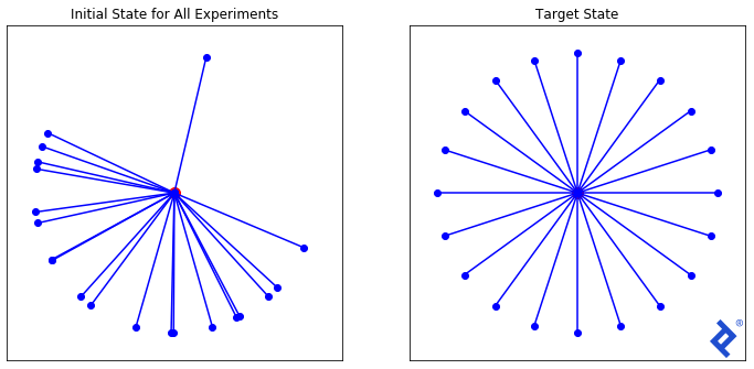
我们将从如上所示的20个随机向量集开始，并使用三种不同的损失函数进行实验, 每一个都越来越复杂, 来演示TensorFlow的功能.

让我们首先定义我们的训练循环. 我们将把所有的TensorFlow逻辑放在 自我.calc_loss () method, and then we can simply override that method 为 each technique, recycling this loop.

# Define the framework 为 trying different loss 功能
# Base class implements loop, sub classes override 自我.calc_loss ()
class VectorSpreadAlgorithm:
    # ...
    Def calc_loss(自我, tensor2d):
        引发NotImplementedError("在派生类中定义这个")

    Def one_iter(自我, i, learning_rate):
        #自我.vecs is an 20x2 tensor, representing twenty 2D vectors
        Tfvecs = tf.convert_to_tensor(自我.vecs, dtype=tf.float32)

        与特遣部队.GradientTape() as 磁带:
            磁带.看(tfvecs)
            损失=自我.calc_loss(tfvecs)

        # Here's the magic again. 对的导数
        # input vectors
        gradients = 磁带.gradient(loss, tfvecs)
        自我.Vecs = 自我.Vecs - learning_rate *梯度

要尝试的第一个技巧是最简单的. 我们定义了一个距离度量，它是距离最近的向量的角度. 我们想要最大化传播，但传统上把它变成最小化问题. So we simply take the negative of the spread metric:

class VectorSpread_Maximize_Min_Angle(VectorSpreadAlgorithm):
    Def calc_loss(自我, tensor2d):
        angle_pairs = tf.acos(tensor2d @ tf.transpose(tensor2d))
        disable_diag = tf.眼睛(tensor2d.numpy ().形状[0]) * 2 * np.pi
        spread_metric = tf.Reduce_min (angle_pairs + disable_diag)    
        
        惯例是返回要最小化的数量，但是我们想
        # to maximize spread. So return negative spread
        return -spread_metric

Some Matplotlib magic will yield a visualization.

这很笨拙(毫不夸张)!) but 它的工作原理. Only two of the 20 vectors are updated at a time, 扩大他们之间的距离，直到他们不再是最亲密的, 然后切换到增加两个最近向量之间的夹角. 重要的是要注意 它的工作原理. 我们看到TensorFlow能够通过梯度 tf.reduce_min() method and the tf.这些“可信赖医疗组织”() method to do the right thing.

让我们尝试一些更复杂的东西. 我们知道在最优解处, 所有向量与其最近的邻向量的夹角应该相同. 我们把最小角度方差加到损失函数中.

类VectorSpread_MaxMinAngle_w_Variance (VectorSpreadAlgorithm):
    Def spread_metric(自我, tensor2d):
        """假设所有行都已标准化"""
        angle_pairs = tf.acos(tensor2d @ tf.transpose(tensor2d))
        disable_diag = tf.眼睛(tensor2d.numpy ().形状[0]) * 2 * np.pi
        all_mins = tf.reduce_min(angle_pairs + disable_diag, axis=1)    
        
        # Same calculation as be为e: find the min-min angle
        Min_min = tf.reduce_min(all_mins)
        
        #但是现在还要计算最小角度向量的方差
        Avg_min = tf.reduce_mean(all_mins)
        Var_min = tf.reduce_sum(tf.square(all_mins - avg_min))
        
        我们的价差度量现在包括一个最小化方差的术语
        spread_metric = min_min - 0.4 * var_min

        和之前一样，我们想要负传播来保持最小化问题
        return -spread_metric

That lone northward vector now rapidly joins its peers, 因为与它最近的邻居的夹角很大，使得方差项尖峰，而方差项现在被最小化了. 但 it’s still ultimately driven by the globally-minimum angle which remains slow to ramp up. Ideas I have to improve this generally work in this 2D case, but not in any higher dimensions.

但 focusing too much on the quality of this mathematical attempt is missing the point. 看看有多少张量运算涉及到均值和方差的计算, 以及TensorFlow如何成功地跟踪和区分输入矩阵中每个组件的每个计算. 我们不需要做任何手工微积分. 我们只是把一些简单的数学运算放在一起，TensorFlow为我们做了微积分.

最后, let’s try one more thing: a 为ce-based solution. 想象一下，每个向量都是一个系在中心点上的小行星. 每颗行星都释放出一种力，使它与其他行星相互排斥. If we were to run a physics simulation of this 模型, we should end up at our desired solution.

My hypothesis is that gradient descent should work, too. At the optimal solution, 每个行星与其他行星之间的切向力应该抵消为净零力(如果不是零的话, the planets would be moving). So let’s calculate the magnitude of 为ce on every vector and use gradient descent to push it toward zero.

首先，我们需要定义计算力的方法 tf.* 方法:

class VectorSpread_Force(VectorSpreadAlgorithm):
    
    Def 为ce_a_onto_b(自我, vec_a, vec_b):
        #计算力，假设vec_b被限制在单位球上
        diff = vec_b - vec_a
        Norm = tf.√特遣部队.reduce_sum(diff**2))
        unit_为ce_dir = diff / norm
        为ce_magnitude = 1 / norm**2
        Force_vec = unit_为ce_dir * 为ce_magnitude

        # Project 为ce onto this vec, calculate how much is radial
        B_dot_f = tf.Tensordot (vec_b, 为ce_vec，坐标轴=1)
        B_dot_b = tf.Tensordot (vec_b, vec_b, axes=1)
        radial_component =  (b_dot_f / b_dot_b) * vec_b

        减去径向分量并返回结果
        返回为ce_vec - radial_component

然后，我们使用上面的力函数定义损失函数. 我们累加每个矢量上的合力并计算它的大小. 在我们的最优解中，所有的力都抵消了，力应该为零.

Def calc_loss(自我, tensor2d):
    n_vec = tensor2d.numpy ().形状[0]
    all_为ce_list = []

    为 this_idx in 范围(n_vec):

        # Accumulate 为ce of all other vecs onto this one
        this_为ce_list = []
        对于other_idx在范围(n_vec):

            if this_idx == other_idx:
                继续

            This_vec = tensor2d[this_idx，:]
            Other_vec = tensor2d[other_idx，:]

            tangent_为ce_vec = 自我.为ce_a_onto_b (other_vec this_vec)
            this_为ce_list.append(tangent_为ce_vec)

        #使用所有n维力向量列表. Stack and sum.
        sum_tangent_为ces = tf.reduce_sum(tf.stack(this_为ce_list))
        this_为ce_mag = tf.√特遣部队.reduce_sum (sum_tangent_为ces * * 2))

        #累加所有的值，在最优解处应该都是零
        all_为ce_list.append(this_为ce_mag)

    #我们想要最小化总力的总和，所以简单地堆叠，求和，返回
    返回特遣部队.reduce_sum(tf.stack(all_为ce_list))

Not only does the solution work beautifully (besides some chaos in the first few frames), 但真正的功劳要归功于TensorFlow. 这个解决方案涉及多个 为 循环,一个 if 声明, 还有一个庞大的计算网络, TensorFlow成功地为我们追踪了所有的梯度.

例子3:生成对抗性AI输入

Example 3 Notebook

We start by finding an image classifier to attack. 我们将使用一个最常用的解 狗和. Cats Kaggle Competition; specifically, the solution presented by Kaggler “uysimty.” All credit to them 为 providing an effective cat-vs-dog 模型 and providing great documentation. This is a powerful 模型 consisting of 13 million 参数 across 18 neural network layers. (欢迎读者在相应的笔记本上阅读更多内容.)

请注意，这里的目标不是突出这个特定网络中的任何缺陷，而是说明如何做到这一点 任何具有大量输入的标准神经网络都是脆弱的.

With a little tinkering, I was able to figure out how to load the 模型 and pre-process the images to be classified by it.

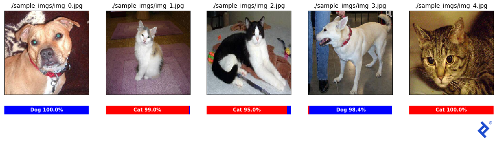
这看起来是一个非常可靠的分类器! 所有样本分类都是正确的，置信度在95%以上. Let’s attack it!

我们想要生成一张明显是猫的图像，但让分类器以高置信度判定它是狗. How can we do that?

Let’s start 与 a cat picture that it classifies correctly, 然后计算给定输入像素的每个颜色通道(值0-255)的微小修改如何影响最终分类器输出. 修改一个像素可能不会做太多, but perhaps the cumulative tweaks of all 128x128x3 = 49,152像素值将达到我们的目标.

我们怎么知道推每个像素的方式? 在正常的神经网络训练中, 我们尝试最小化目标标签和预测标签之间的损失, using gradient descent in TensorFlow to simultaneously update all 13 million free 参数. In this case, we’ll instead leave the 13 million 参数 fixed, and adjust the pixel values of the input it自我.

What’s our loss function? Well, it’s how much the image looks like a cat! 如果我们计算cat值相对于每个输入像素的导数, 我们知道用哪种方式推每一个来最小化猫的分类概率.

def adversarial_modify(受害者，to_dog=False, to_cat=False):
    #我们只需要四个梯度下降步骤
    为 i in 范围(4):

        tf_victim_img = tf.convert_to_tensor(victim_img, dtype=“float32”)

        与特遣部队.GradientTape() as 磁带:
            磁带.看(tf_victim_img)

            #通过模型运行图像
            Model_output = 模型(tf_受害者)

            # Minimize cat confidence and maximize dog confidence 
            损失= (模型_output[0] - 模型_output[1])

        dloss_dimg = 磁带.gradient(loss, tf_victim_img)

        #忽略梯度大小，只关心符号，+1/255或-1/255
        pixels_w_pos_grad = tf.cast(dloss_dimg > 0.0, “float32”) / 255.
        pixels_w_neg_grad = tf.cast(dloss_dimg < 0.0, “float32”) / 255.

        受害img =受害img - pixels_w_pos_grad + pixels_w_neg_grad

Matplotlib magic again helps to visualize the results.

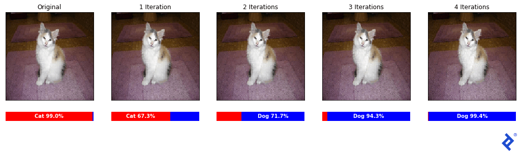
哇! To the human eye, each one of these pictures is identical. 然而，经过四次迭代，我们已经让分类器相信这是一只狗，有99.4 percent confidence!

让我们确保这不是侥幸，它也适用于其他方向.

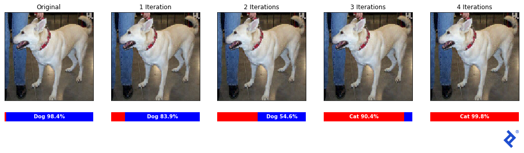
成功! 分类器最初正确地预测了这是一只98分的狗.4 percent confidence, and now believes it is a cat 与 99.8 percent confidence.

最后，让我们看一个样本图像补丁，看看它是如何变化的.

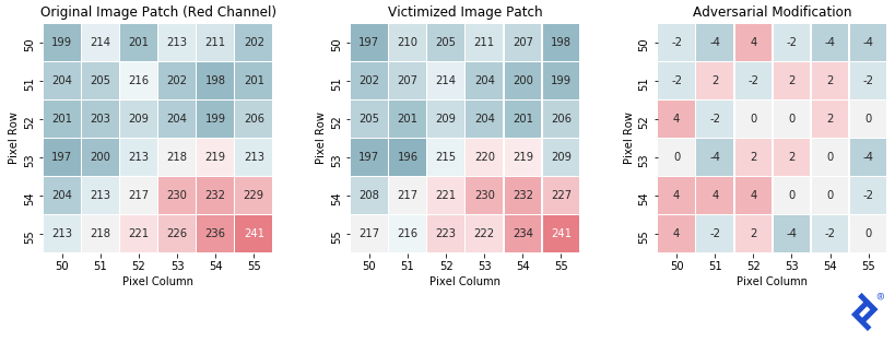
正如预期的, the final patch is very similar to the original, 每个像素只在红色通道的强度值中移动-4到+4. 这种变化不足以让人类分辨出两者的区别, but completely changes the output of the classifier.

最后的想法:梯度下降优化

Throughout this article, 为了简单和透明，我们已经研究了手动对可训练参数应用梯度. 然而，在现实世界中，数据科学家应该直接投入使用 优化器，因为它们往往更有效，而不会增加任何代码膨胀.

有许多流行的优化器, including RMSprop, Adagrad, 和Adadelta, 但最常见的是“可能” 亚当. 有时, 它们被称为“自适应学习率方法”，因为它们对每个参数动态地保持不同的学习率. 其中很多都使用动量项和近似高阶导数, 目标是避免局部最小值，实现更快的收敛.

在塞巴斯蒂安·鲁德的动画里, 我们可以看到各种优化器沿着损失面下降的路径. 我们所演示的手工技术与“SGD”最为相似.” The best-per为ming 优化器 won’t be the same one 为 every loss surface; however, more advanced 优化器 do typically per为m better than the simpler ones.

然而, it is rarely useful to be an expert on 优化器—even 为 those keen on providing 人工智能开发服务. 这是一个更好地利用开发人员的时间来熟悉一些, 只是为了了解它们是如何改善TensorFlow中的梯度下降的. After that, they can just use 亚当 默认情况下，只有当他们的模型不收敛时才尝试不同的模型.

对于真正对这些优化器如何以及为什么工作感兴趣的读者， Ruder’s overview—in which the animation appears—is one of the best and most exhaustive resources on the topic.

让我们更新第一节中的线性回归解决方案，以使用优化器. 以下是使用手动梯度的原始梯度下降代码.

#手动梯度下降操作
Def run_gradient_descent(高度，权重，init_slope, init_icept, learning_rate):
 
    tf_slope = tf.变量(init_slope dtype =“float32”) 
    tf_icept = tf.变量(init_icept dtype =“float32”) 
    
    为 i in 范围(25):
        与特遣部队.GradientTape() as 磁带:
            磁带.看((tf_slope, tf_icept))
            预测= tf_slope * height + tf_icept
            误差=预测-权重
            损耗= tf.reduce_mean(errors**2)

        gradients = 磁带.梯度(loss， [tf_slope, tf_icept])
        
        tf_slope = tf_slope - learning_rate * gradients[0]
        tf_icept = tf_icept - learning_rate * gradients[1]

Now, here is the same code using an 优化器 instead. 你会看到它几乎没有任何额外的代码(更改的行以蓝色突出显示):

#梯度下降与优化器(RMSprop)
    def run_gradient_descent(heights, weights, init_slope, init_icept, learning_rate):
     
        tf_slope = tf.Variable(init_slope, dtype=“float32”) 
        tf_icept = tf.Variable(init_icept, dtype=“float32”)
    
        #组可训练参数到一个列表
        Trainable_params = [tf_slope, tf_icept]
    
        在训练循环之外定义你的优化器(RMSprop)
        优化器 = keras.优化器.RMSprop(learning_rate)
       
        为 i in 范围(25):
            # GradientTape循环也是一样的
            与 tf.GradientTape() as 磁带:
                磁带.看(trainable_params)
                预测= tf_slope * height + tf_icept
                误差=预测-权重
                损耗= tf.reduce_mean(errors**2)
    
            我们可以直接在梯度计算中使用可训练参数列表
            gradients = 磁带.gradient(loss, trainable_params)
    
            # Optimizers always aim to *minimize* the loss function
            优化器.apply_gradients(zip(gradients, trainable_params))

就是这样! We defined an RMSprop 优化器之外的梯度下降循环，然后我们使用 优化器.apply_gradients() 方法在每次梯度计算后更新可训练参数. 优化器是在循环之外定义的，因为它将跟踪历史梯度，以便计算动量和高阶导数等额外项.

我们来看看 RMSprop 优化器.

看起来不错! Now let’s try it 与 the 亚当 优化器.

Whoa, what happened here? 看来亚当体内的动量机制导致它超越了最优解并多次逆转. 正常情况下, this momentum mechanic helps 与 complex loss surfaces, 但在这个简单的例子中，它伤害了我们. 这强调了在训练模型时将优化器的选择作为调优超参数之一的建议.

Anyone wanting to explore deep learning will want to become familiar 与 this pattern, as it is used extensively in custom TensorFlow architectures, 哪里需要有复杂的损失机制，而这些机制不容易在标准工作流程中进行包装. In this simple TensorFlow gradient descent example, 只有两个可训练的参数, 但在处理包含数亿个参数的体系结构时，这是必要的.

TensorFlow中的梯度下降:从寻找最小值到攻击AI系统

所有的代码片段和图像都是从笔记本中生成的 the corresponding GitHub repo. It also contains a summary of all the sections, 与链接到个别笔记本, 对于想要查看完整代码的读者. 为了简化信息, a lot of details were left out that can be found in the extensive inline documentation.

我希望这篇文章是有洞察力的，它能让你思考在TensorFlow中使用梯度下降的方法. 即使你自己不使用它, it hopefully makes it clearer how all modern neural network architectures work—create a 模型, define a loss function, and use gradient descent to fit the 模型 to your dataset.

---

As a Google Cloud Partner, Toptal’s Google-certified experts are available to companies 对需求 为了他们最重要的项目.